In earlier posts, I discussed why LFM’s are necessary, and key issues to consider when building them:
— Which horizons to include
— Which wells to include
— How to populate the log data
Today, I share some thoughts on selecting wells and populating them into 3D low frequency models.
My main point on selecting wells: choose as few as possible. On tightly focused projects, I might even build a homogenous model with only one well. A great way to reduce uncertainties! (Although the logs could still be inaccurate, or with a bad time-depth relationship…so there are always errors and uncertainties.)
From yesterday’s post, the image from Rizwan and Akhter (Open Geosciences 2021) seems to show a model with only 1 well. This can be quite effective!
With early exploration, however, you might have access to 2 or 3 wells, with good distance in between; in this case, I’d use all three – or, if the situation permits, build three small homogenous models centered on each of them.
With development, you might have dozens of wells, quite close together – but it’s rare if they have full and calibrated log suites. Too many uncertainties! To minimize this, I’d carefully select only a few key wells (mostly within the reservoir, with good log suites, and straight holes if possible), and leave the remaining as validation points.
Here’s a comparison of a LFM filtered to the necessary bandwidth (approximately 0-6 Hz) (left panel) vs. the final inversion with low frequency model (approximately 0-45 Hz) (right panel). (own work)
Now it’s time to populate the log data – how best to do this? Simple mathematical interpolations are quick and easy – but always wrong to some degree. Populating with trends like attribute weighting maps helps, but it’s labor intensive – and still has uncertainties. New tools with AI and multi-attribute interpolations show great promise.
Bottom line: there’s no “right” way to populate models – remember, they’re all just predictions. The “right” choice will vary by scenario.
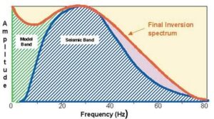
What about supplementing the lowest frequencies (~0-2 Hz) of your model with seismic velocities? Yes of course, but seismic velocity analysis has its own uncertainties, plus you must convert the vels to impedance with a velocity-density relationship (with its own uncertainties) – and even then, a bandwidth gap still remains to be filled by the populated well logs. (In recent years, FWI velocity models generated to higher frequencies can contribute tremendously – but they’re quite expensive!)
Conclusion – with this series of posts, I’ve confirmed why LFMs are necessary for inversion, but they inevitably introduce uncertainties. You can never remove all doubt, but there are ways to minimize uncertainties. I find the most effective approach is to keep your models as small and simple as possible.
Below is a nice illustration of how a good LF model influences the final inverted impedance (own work).
Thanks for reading these posts! Let me know of any thoughts or questions. Maybe next I’ll talk about other strategies and pitfalls for seismic inversion.