Lately I’ve been thinking about low frequencies, in the context of seismic inversion and low frequency models (LFMs).
There are many great posts on LinkedIn, plus tons of good articles online. Today I’ll start a little series of posts with thoughts on LFM’s.
WHY LOW FREQUENCY MODELS?
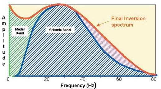
Since seismic data is bandlimited (no signal below ~6-10 Hz) and inversion algorithms operate on “full-bandwidth” solutions (meaning, 0 Hz up to the top of input seismic bandwidth), most algorithms require elastic property trends or models to “fill in” the low frequencies missing from the seismic. We call these low frequency models (LFMs).
The image below shows the different components of an inversion product, in frequency-amplitude space. The blue = seismic data, green = LFM, and red = the bandwidth of the final product (from Pendrel and Van Reil, CSEG Recorder, 2000).
Post-stack inversions derive p-impedance from the seismic, so the algorithm requires an input p-impedance LFM; pre-stack inversions require models of p-impedance, s-impedance and VpVs (or variants thereof).
LFMs are essential to quantitative interpretation, as any inverted elastic property without restored low frequencies is “bandlimited” and only qualitative, with no way to directly calibrate with well control. We want quantitative, and this requires restoring low frequencies.
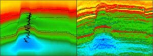
But – as important as they are – LFMs are the greatest source of uncertainty for seismic inversions. These “starting models” are usually constructed of log data from available wells, populated in some manner into a 3D volume, guided along structure by horizons and faults. Their effectiveness is typically based on three key factors:
— Which horizons to include
— Which wells to include
— How to populate the log data
In my decades of experience with seismic inversions, I’ve uncovered a few tricks to help minimize uncertainties related to LFMs. Starting tomorrow, I’ll address the three key factors with some of my experiences. Stay tuned.